Introducing a Simpler Way to get IP Address Data in Snowflake

We’ve just launched a new way to access our data in Snowflake in a really quick and intuitive way, leveraging Snowflake’s powerful UDTFs.

The backstory: Joining IPs to geolocation

One of the challenges, when we launched our data on the Snowflake Marketplace, was to make the lookups of our data performant.

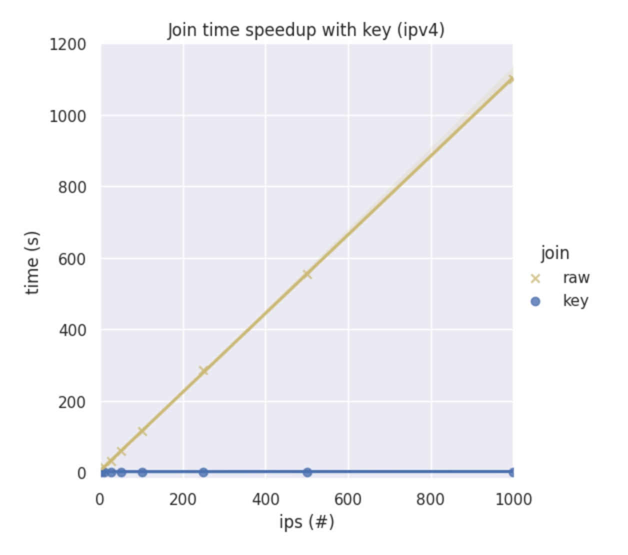
Because our data maps to IP ranges, rather than specific IPs, range joins can be slow. That's why we created an optimized version. By splitting the data and creating a join key, you can now do an exact join.

In the past, BETWEEN was the intuitive way to conduct raw joins. The problem is that this scales badly. The result is that we get a lot of support requests from users asking to help them to figure out why their queries are slow.

For instance, here's how the raw basic join and join_key join compare for IPv4 addresses.

And here's how these joins compare for IPv6 addresses.

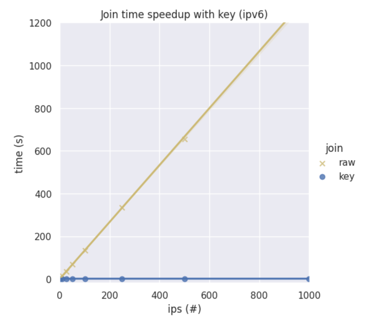
In short, our new join key is now the quickest way to conduct a query.

How we simplified IP address queries in Snowflake

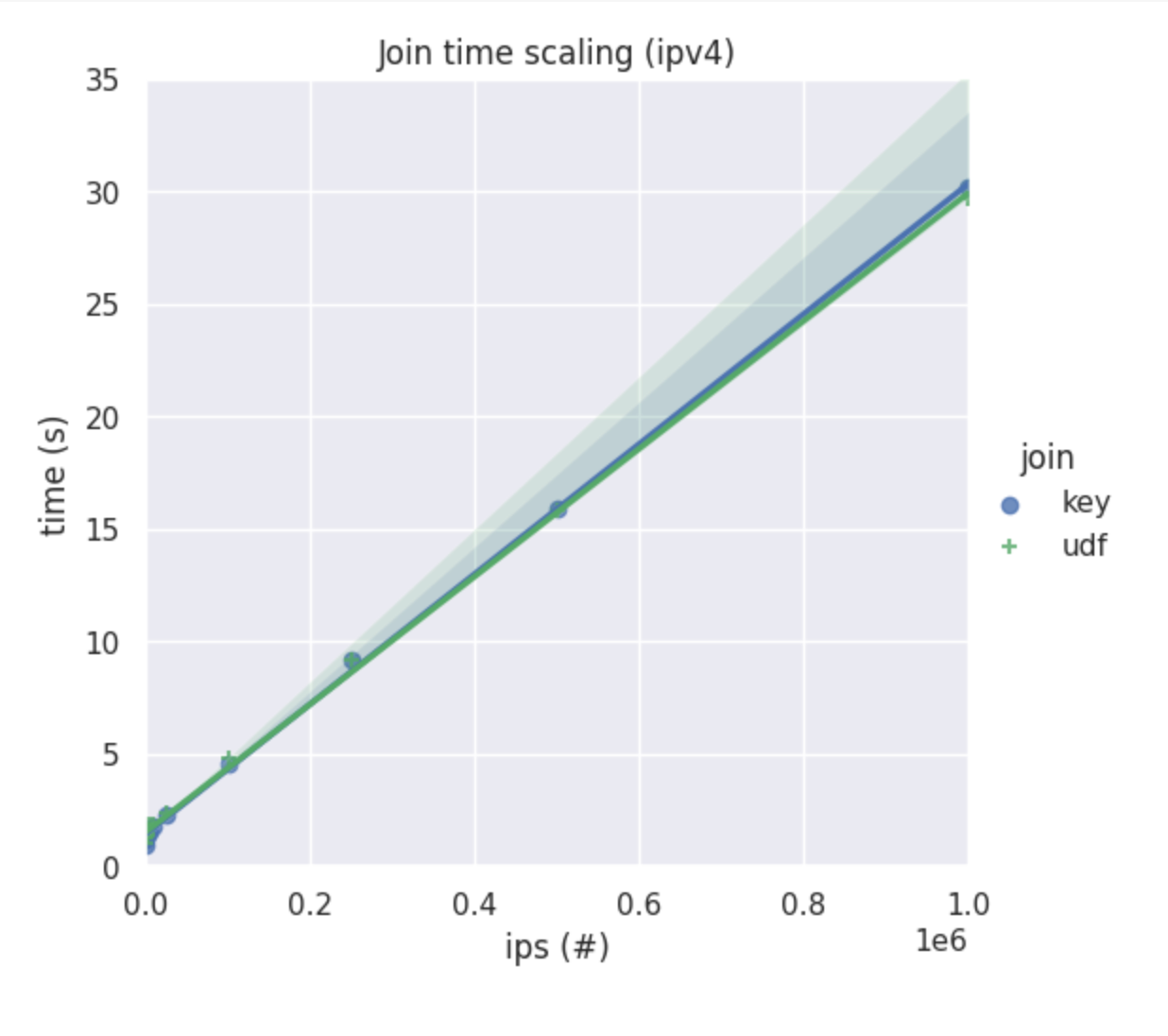
Using the join_key join form will make queries incredibly fast. But all of this would be much better if users didn’t need to worry about the details of how our data is stored or about making the join performant at all in the first place.

With these new UDTFs, users are able to enrich any IP address within Snowflake with our IP geolocation, company, carrier & VPN detection data sets with a simple call to our function - no need to think about using or understanding how to use join_key directly.

It works with IPv4 and IPv6 addresses and scales to massive data sets as represented by the graph below

Examples

Here's a basic example of the data retrieved by the ip_country function.

And here's a sample of an ip_location query:

CREATE OR REPLACE FUNCTION ip_location(ip text)
RETURNS TABLE (
  city text,
  region text,
  country text,
  postal text,
  lat float,
  lng float,
  timezone text
) AS
'SELECT
  city,
  region,
  country,
  postal,
  lat,
  lng,
  timezone
FROM location
WHERE join_key = to_join_key(ip)
AND to_int(ip) BETWEEN start_ip_int AND end_ip_int';

SELECT *
FROM (
  SELECT ip
  FROM sample_ips
) a
JOIN TABLE (ip_location(a.ip)) i;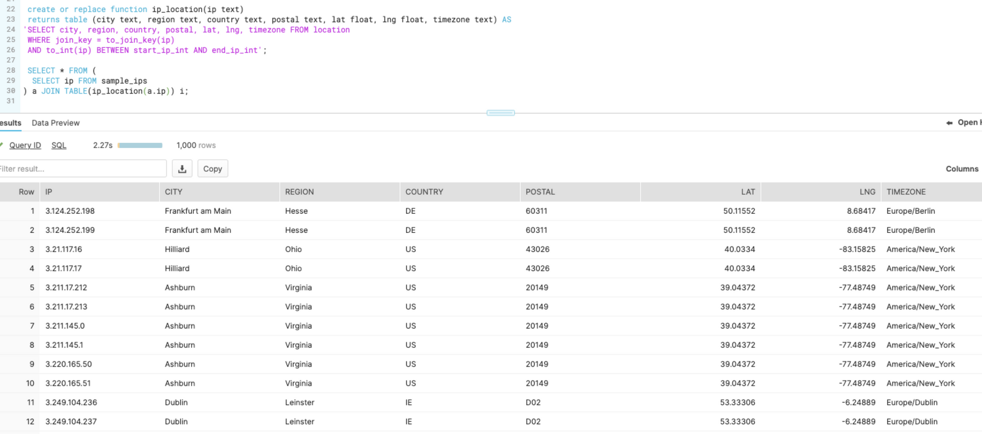

The functions we’ve launched are:

• ip_asn
• ip_carrier
• ip_company
• ip_location
• ip_privacy

Each function returns a full set of fields from our corresponding data set, and each works with IPv4 and IPv6.

Some useful links:

1. Docs: https://ipinfo.io/integrations/snowflake
2. IP Geolocation: https://app.snowflake.com/marketplace/listing/GZSTZ3VDMFI/ipinfo-ipinfo-geolocation-ip-address-data
3. ASN: https://app.snowflake.com/marketplace/listing/GZSTZ3VDMFM/ipinfo-ipinfo-asn-data
4. IP to company: https://app.snowflake.com/marketplace/listing/GZSTZ3VDMEX/ipinfo-ipinfo-company-ip-address-data
5. Privacy Detection: https://app.snowflake.com/marketplace/listing/GZSTZ3VDMFU/ipinfo-ipinfo-ip-address-data-for-privacy-detection-vpn-tor-relay-proxy-etc

How to use these functions for data enrichment

Let’s get into an example of using these functions to enrich some sample data in Snowflake, and show what we can do with the results.

Assume you have a table called logs and it has some column ip that stores the string form of an IPv4 or IPv6 address. The following easy-to-understand query would perform a join between your log data and 3 different IP datasets - geolocation, ASN & privacy.

SELECT * FROM logs l
JOIN TABLE(ip_location(l.ip))
JOIN TABLE(ip_asn(l.ip))
JOIN TABLE(ip_privacy(l.ip))

This would generate a table containing first the columns of your log data, including the IP, and then all the columns available from the geolocation, ASN & privacy datasets.

How we developed these functions

While the whole point of this article is to tell users to "just call the function", we're aware that some of you enjoy the technical details. This is for you. Here's how and why we created the join key functions.

After receiving reports from users that our sample queries were slow, we started investigating the issue.

Step 1: Replicate the issue

We also noticed several forums that mentioned similar issues, such as these.

• How can I efficiently transform a two-column range into an expanded table?
• Performance of LEFT JOIN ON left.col1 between right.colA and right.colB
• Snowflake improve search join IP over Network
• Geolocation of IP Addresses in Snowflake

Here's the code we used to replicate the issue reported by Snowflake users.

We noticed that we should pre-split all the ranges to /16s and also write the join key to the table, so the user just needs to do the transform to a /16 once. At this point, we also decided we could make the query even more simple for users by creating a UDF.

Step 2: Develop a UDF

When we created this function,

CREATE FUNCTION ip_to_joinkey(ip text)
  RETURNS variant
  as
  $$
    parse_ip(CONCAT(ip, '/16'), 'inet''):ipv4_range_start
  $$
  ;
-- SELECT ip_to_joinkey('8.8.8.8');
-- => 123742016

We discovered some issues with the BQ export and file uploads. Additionally, we realized that Snowflake UDFs are more powerful than BQ functions (eg. can return tables).

Using Snowflake's Tabular SQL UDFs guide, we developed a basic working example that might port to IPs.

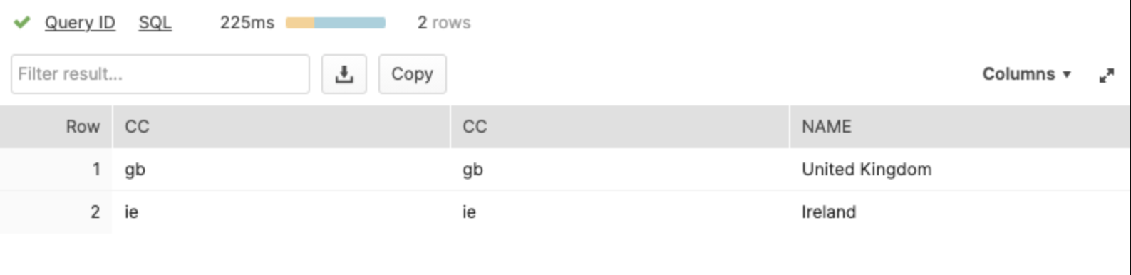
CREATE TABLE countries (cc text, name text);
INSERT INTO
countries VALUES ('gb', 'United Kingdom'), ('us', 'United States'), ('ru', 'Russia'), ('ie', 'Ireland'); //...
SELECT name FROM countries WHERE cc = 'gb';

CREATE OR REPLACE FUNCTION get_cc(cc text)
RETURNS TABLE(cc text, name text)
AS '
  SELECT *
  FROM countries c
  WHERE c.cc = cc
  ';

SELECT * FROM TABLE(get_cc('gb'));

CREATE TABLE codes (cc text);
INSERT INTO
codes VALUES ('gb'), ('ie');
SELECT *
FROM codes c
JOIN TABLE (get_cc(cc)) x;

This returned these results.

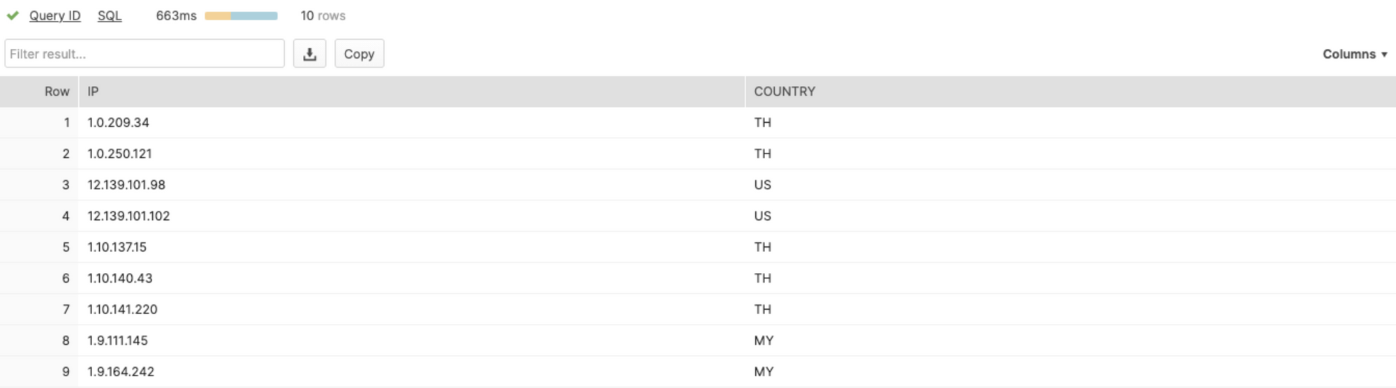
At this point, we tried a basic IP example with a join. Here's what it returned.

Step 3: Create functions and let users test them

Now that we knew this was going to solve a lot of issues for Snowflake users and for Snowflake engineers demo-ing their product for customers, we started building out these different functions.

• ip_asn
• ip_carrier
• ip_company
• ip_location
• ip_privacy

We did run into a few issues when we tried granting permissions to share the function with new users. At this point, we needed to create a Stored Procedure to grant permissions on all newly created UDFs. This reduced our efforts of granting permissions to each and every UDF manually.

Step 4: Gather performance metrics

We also wanted to conduct detailed performance comparisons of simple join, join_key join, and UDF. To start, we created a bigger sample IP table. Initially, we conducted our tests with IPv4 addresses.

These numbers confirmed that UDF doesn't have a ton of overhead compared to the raw join_key join. (Note: See the graphs at the beginning of this article to compare the results for yourself.)

The end result is that users never need to do a basic join. They might as well use UDFs because they're just as fast (if not slightly faster) than using the join key raw. Additionally, they're much easier to read.

As with all of our supported integrations, our data experts are ready to answer questions or listen to your feedback. We’d love to hear from you!